Learning Latent Dynamics for
Planning from Pixels
Abstract
Planning has been very successful for control tasks with known environment dynamics. To leverage planning in unknown environments, the agent needs to learn the dynamics from interactions with the world. However, learning dynamics models that are accurate enough for planning has been a long-standing challenge, especially in image-based domains. We propose the Deep Planning Network (PlaNet), a purely model-based agent that learns the environment dynamics from images and chooses actions through fast online planning in latent space. To achieve high performance, the dynamics model must accurately predict the rewards ahead for multiple time steps. We approach this problem using a latent dynamics model with both deterministic and stochastic transition components and a multi-step variational inference objective that we call latent overshooting. Using only pixel observations, our agent solves continuous control tasks with contact dynamics, partial observability, and sparse rewards, which exceed the difficulty of tasks that were previously solved by planning with learned models. PlaNet uses substantially fewer episodes and reaches final performance close to and sometimes higher than strong model-free algorithms. The source code is available as open source for the research community to build upon.
Introduction
Planning is a natural and powerful approach to decision making problems with known dynamics, such as game playing and simulated robot control
Planning using learned models offers several benefits over model-free reinforcement learning. First, model-based planning can be more data efficient because it leverages a richer training signal and does not require propagating rewards through Bellman backups. Moreover, planning carries the promise of increasing performance just by increasing the computational budget for searching for actions, as shown by
Recent work has shown promise in learning the dynamics of simple low-dimensional environments
In this paper, we propose the Deep Planning Network (PlaNet), a model-based agent that learns the environment dynamics from pixels and chooses actions through online planning in a compact latent space. To learn the dynamics, we use a transition model with both stochastic and deterministic components and train it using a generalized variational objective that encourages multi-step predictions. PlaNet solves continuous control tasks from pixels that are more difficult than those previously solved by planning with learned models.
Key contributions of this work are summarized as follows:
-
Planning in latent spaces We solve a variety of tasks from the DeepMind control suite, by learning a dynamics model and efficiently planning in its latent space. Our agent substantially outperforms the model-free A3C and in some cases D4PG algorithm in final performance, with on average 50× less environment interaction and similar computation time.
-
Recurrent state space model We design a latent dynamics model with both deterministic and stochastic components
. Our experiments indicate having both components to be crucial for high planning performance. -
Latent overshooting We generalize the standard variational bound to include multi-step predictions. Using only terms in latent space results in a fast and effective regularizer that improves long-term predictions and is compatible with any latent sequence model.
Latent Space Planning
To solve unknown environments via planning, we need to model the environment dynamics from experience. PlaNet does so by iteratively collecting data using planning and training the dynamics model on the gathered data. In this section, we introduce notation for the environment and describe the general implementation of our model-based agent. In this section, we assume access to a learned dynamics model. Our design and training objective for this model are detailed later on in the Recurrent State Space Model and Latent Overshooting sections respectively.
Problem setup Since individual image observations generally do not reveal the full state of the environment, we consider a partially observable Markov decision process (POMDP). We define a discrete time step , hidden states , image observations , continuous action vectors , and scalar rewards , that follow the stochastic dynamics:
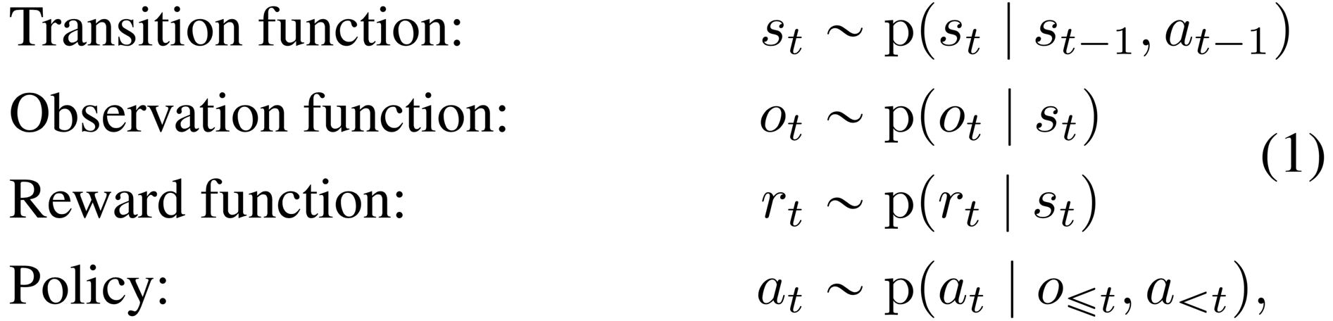
where we assume a fixed initial state without loss of generality. The goal is to implement a policy that maximizes the expected sum of rewards , where the expectation is over the distributions of the environment and the policy.

Model-based planning PlaNet learns a transition model , observation model , and reward model from previously experienced episodes (note italic letters for the model compared to upright letters for the true dynamics). The observation model provides a training signal but is not used for planning. We also learn an encoder to infer an approximate belief over the current hidden state from the history using filtering. Given these components, we implement the policy as a planning algorithm that searches for the best sequence of future actions. We use model-predictive control (MPC)

Experience collection Since the agent may not initially visit all parts of the environment, we need to iteratively collect new experience and refine the dynamics model. We do so by planning with the partially trained model, as shown in Algorithm 1. Starting from a small amount of seed episodes collected under random actions, we train the model and add one additional episode to the data set every update steps. When collecting episodes for the data set, we add small Gaussian exploration noise to the action. To reduce the planning horizon and provide a clearer learning signal to the model, we repeat each action times, as is common in reinforcement learning
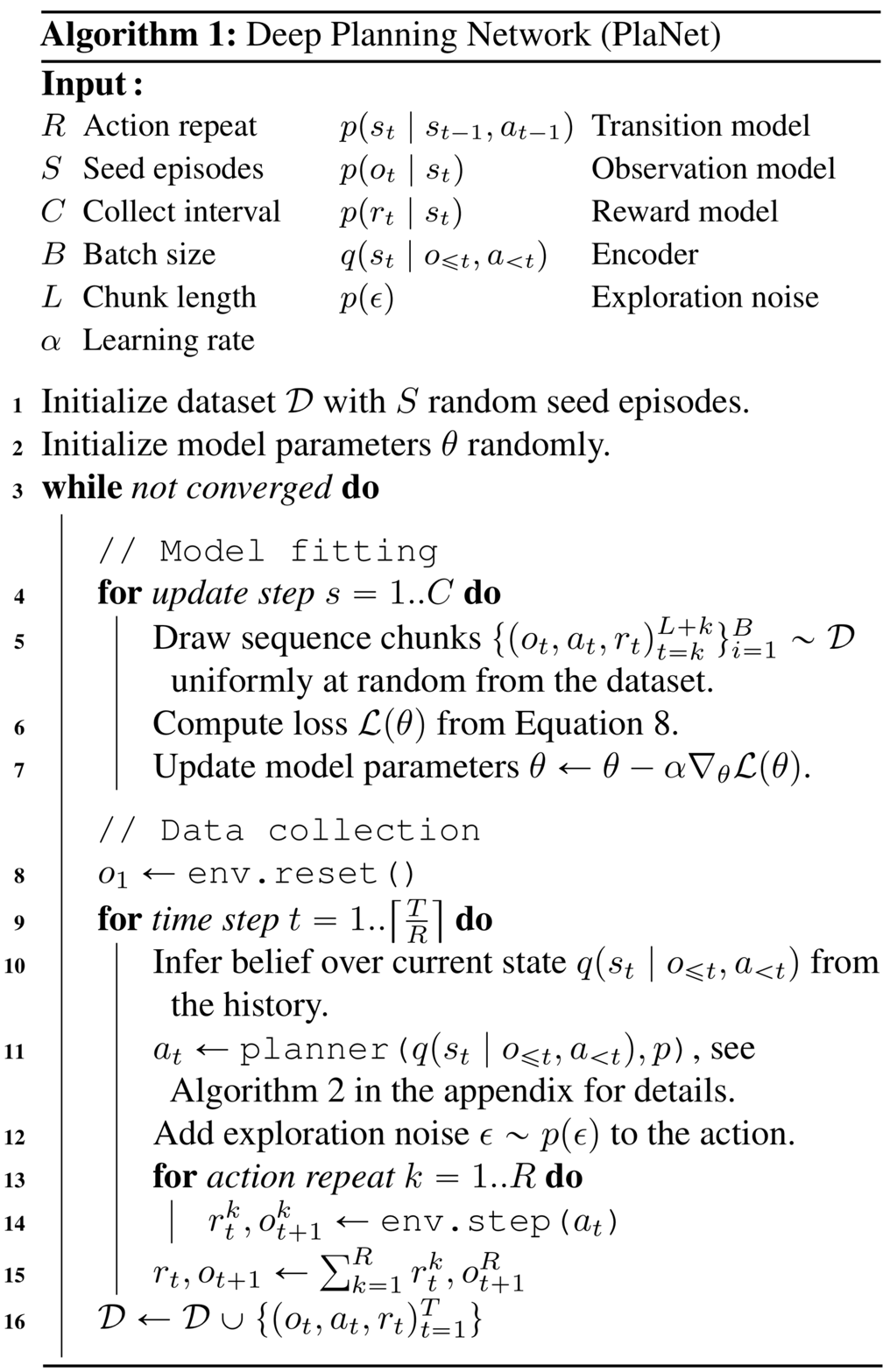
Planning algorithm We use the cross entropy method (CEM)
To evaluate a candidate action sequence under the learned model, we sample a state trajectory starting from the current state belief, and sum the mean rewards predicted along the sequence. Since we use a population-based optimizer, we found it sufficient to consider a single trajectory per action sequence and thus focus the computational budget on evaluating a larger number of different sequences. Because the reward is modeled as a function of the latent state, the planner can operate purely in latent space without generating images, which allows for fast evaluation of large batches of action sequences. The next section introduces the latent dynamics model that the planner uses.
Recurrent State Space Model
For planning, we need to evaluate thousands of action sequences at every time step of the agent. Therefore, we use a recurrent state-space model (RSSM) that can predict forward purely in latent space, similar to recently proposed models
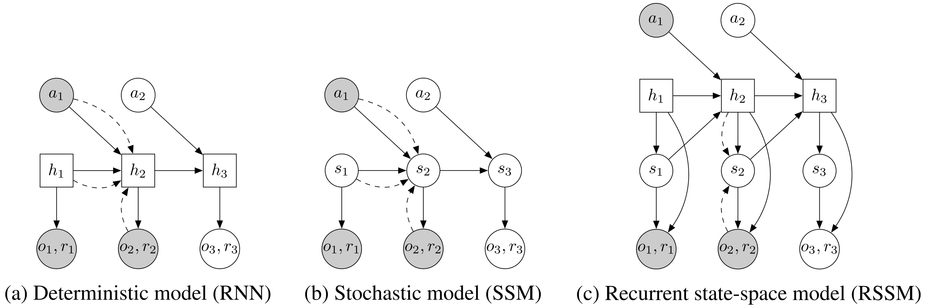
(b) Transitions in a state-space model are purely stochastic. This makes it difficult to remember information over multiple time steps.
(c) We split the state into stochastic and deterministic parts, allowing the model to robustly learn to predict multiple futures.
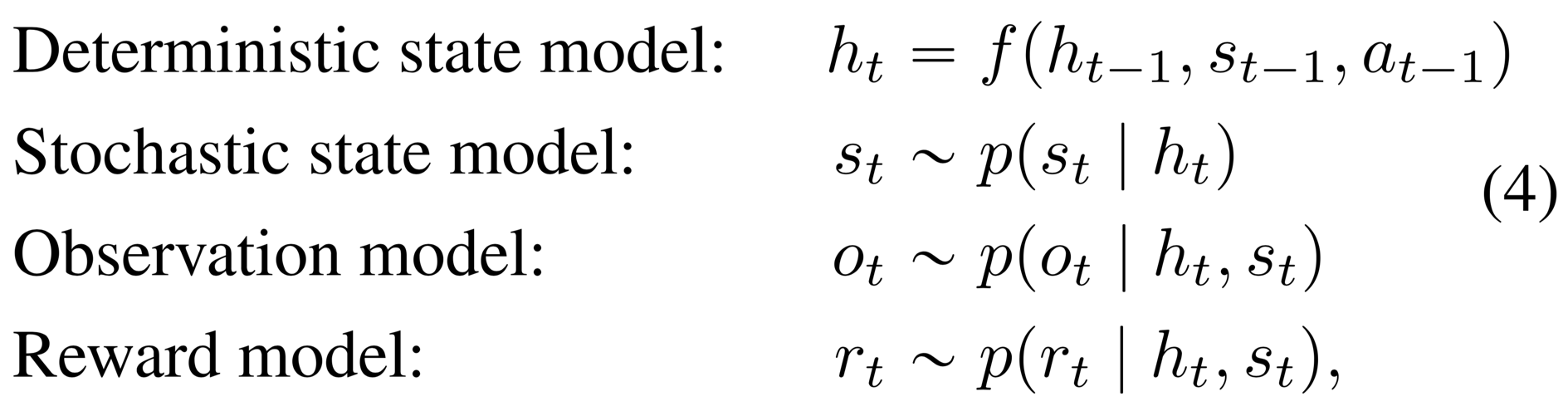
Latent dynamics We consider sequences with discrete time step , high-dimensional image observations , continuous action vectors , and scalar rewards . A typical latent state-space model is shown in Figure 4b and resembles the structure of a partially observable Markov decision process. It defines the generative process of the images and rewards using a hidden state sequence ,
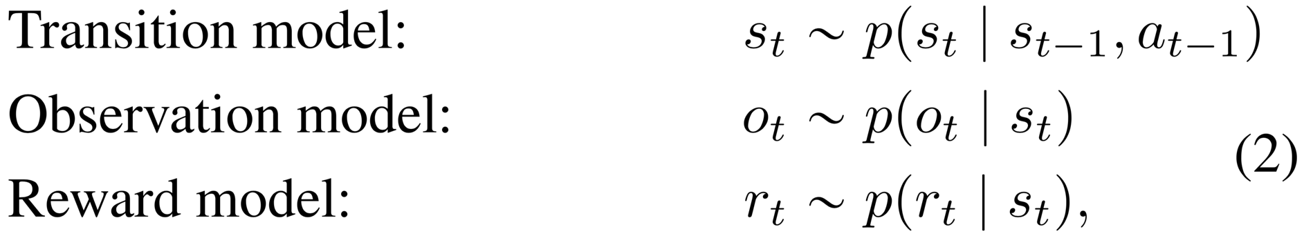
where we assume a fixed initial state without loss of generality. The transition model is Gaussian with mean and variance parameterized by a feed-forward neural network, the observation model is Gaussian with mean parameterized by a deconvolutional neural network and identity covariance, and the reward model is a scalar Gaussian with mean parameterized by a feed-forward neural network and unit variance. Note that the log-likelihood under a Gaussian distribution with unit variance equals the mean squared error up to a constant.
Variational encoder Since the model is non-linear, we cannot directly compute the state posteriors that are needed for parameter learning. Instead, we use an encoder to infer approximate state posteriors from past observations and actions, where is a diagonal Gaussian with mean and variance parameterized by a convolutional neural network followed by a feed-forward neural network. We use the filtering posterior that conditions on past observations since we are ultimately interested in using the model for planning, but one may also use the full smoothing posterior during training
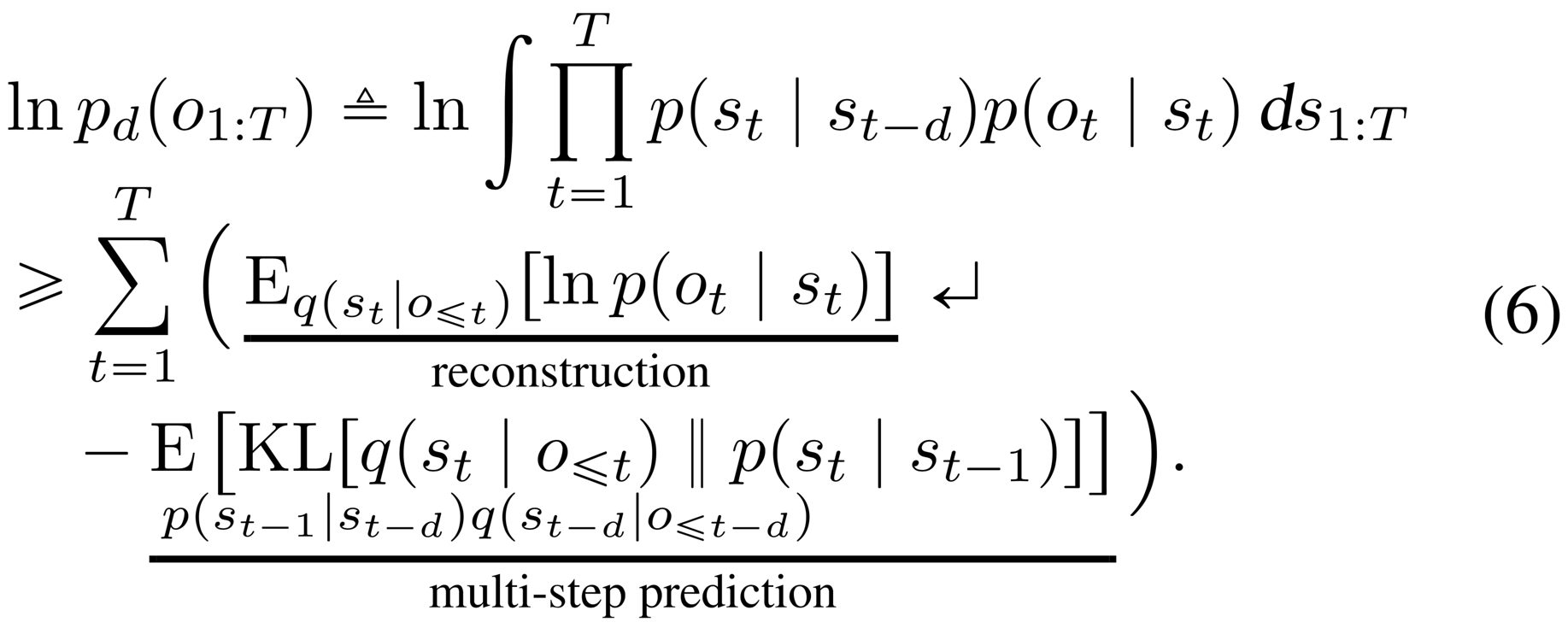
Training objective Using the encoder, we construct a variational bound on the data log-likelihood. For simplicity, we write losses for predicting only the observations -- the reward losses follow by analogy. The variational bound obtained using Jensen's inequality is
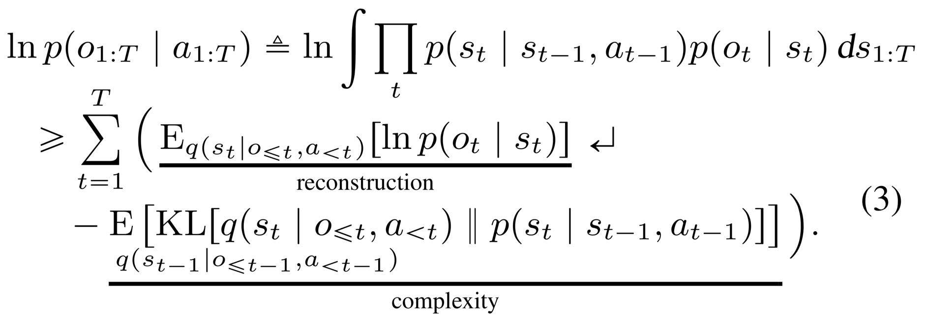
For the derivation, please see the appendix in the PDF. Estimating the outer expectations using a single reparameterized sample yields an efficient objective for inference and learning in non-linear latent variable models that can be optimized using gradient ascent
Deterministic path Despite its generality, the purely stochastic transitions make it difficult for the transition model to reliably remember information for multiple time steps. In theory, this model could learn to set the variance to zero for some state components, but the optimization procedure may not find this solution. This motivates including a deterministic sequence of activation vectors , that allow the model to access not just the last state but all previous states deterministically
where is implemented as a recurrent neural network (RNN). Intuitively, we can understand this model as splitting the state into a stochastic part and a deterministic part , which depend on the stochastic and deterministic parts at the previous time step through the RNN. We use the encoder to parameterize the approximate state posteriors. Importantly, all information about the observations must pass through the sampling step of the encoder to avoid a deterministic shortcut from inputs to reconstructions.
Global prior The model can be trained using the same loss function (Equation 3). In addition, we add a fixed global prior to prevent the posteriors from collapsing in near-deterministic environments. This alleviates overfitting to the initially small training data set and grounds the state beliefs (since posteriors and temporal priors are both learned, they could drift in latent space). The global prior adds additional KL-divergence loss terms from each posterior to a standard Gaussian. Another interpretation of this is to define the prior at each time step as product of the learned temporal prior and the global fixed prior. In the next section, we identify a limitation of the standard objective for latent sequence models and propose a generalization of it that improves long-term predictions.
Latent Overshooting
In the previous section, we derived the typical variational bound for learning and inference in latent sequence models (Equation 3). As show in Equation 3, this objective function contains reconstruction terms for the observations and KL-divergence regularizers for the approximate posteriors. A limitation of this objective is that the transition function is only trained via the KL-divergence regularizers for one-step predictions: the gradient flows through directly into but never traverses a chain of multiple . In this section, we generalize this variational bound to latent overshooting, which trains all multi-step predictions in latent space.
Limited capacity If we could train our model to make perfect one-step predictions, it would also make perfect multi-step predictions, so this would not be a problem. However, when using a model with limited capacity and restricted distributional family, training the model only on one-step predictions until convergence does in general not coincide with the model that is best at multi-step predictions. For successful planning, we need accurate multi-step predictions. Therefore, we take inspiration from
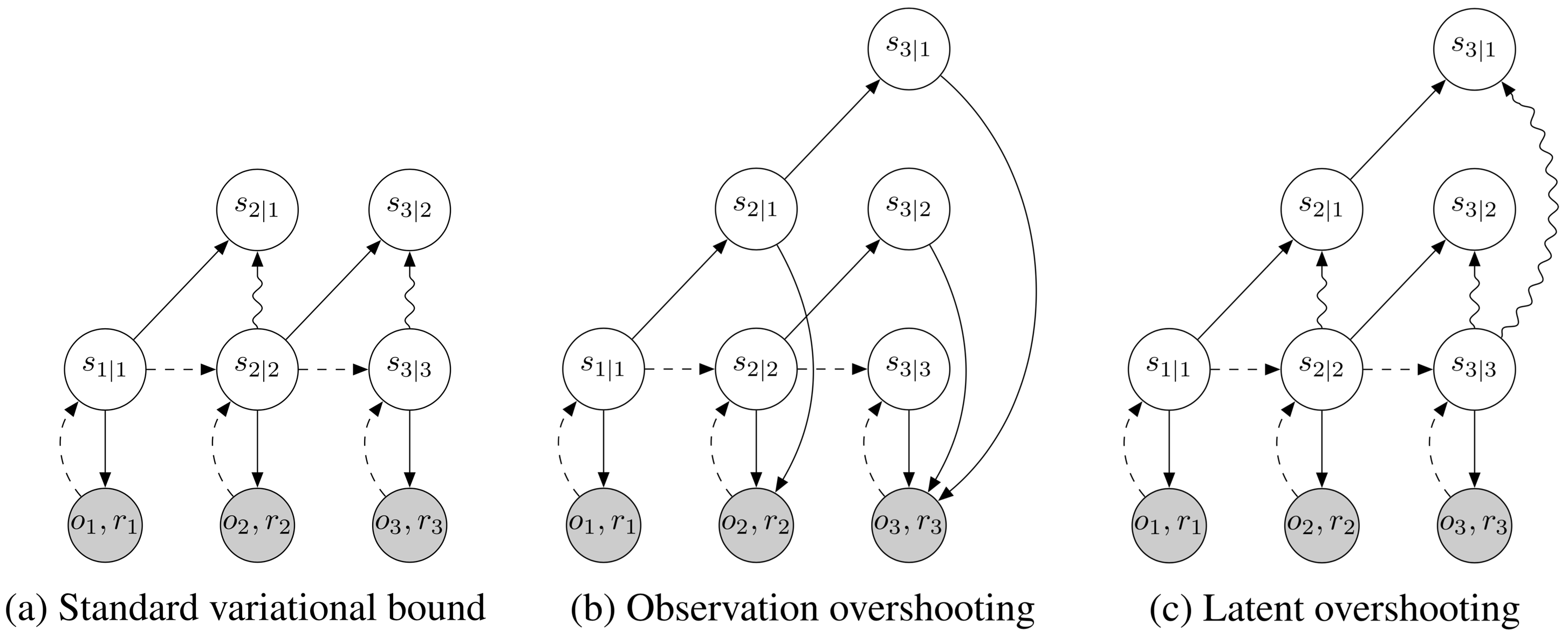
(b) Observation overshooting
(c) Latent overshooting predicts all multi-step priors. These state beliefs are trained towards their corresponding posteriors in latent space to encourage accurate multi-step predictions.
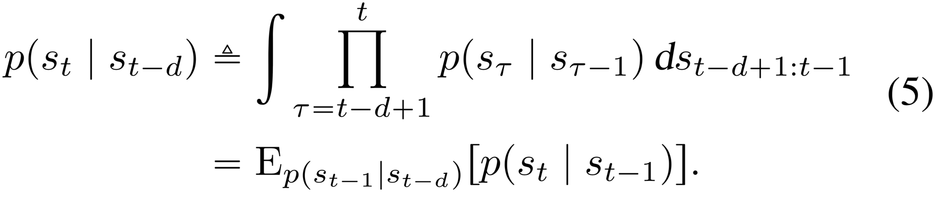
Multi-step prediction We start by generalizing the standard variational bound (Equation 3) from training one-step predictions to training multi-step predictions of a fixed distance . For ease of notation, we omit actions in the conditioning set here; every distribution over is conditioned upon . We first define multi-step predictions, which are computed by repeatedly applying the transition model and integrating out the intermediate states,
The case recovers the one-step transitions used in the original model. Given this definition of a multi-step prediction, we generalize Equation 3 to the variational bound on the multi-step predictive distribution ,
For the derivation, please see the appendix in the PDF. Maximizing this objective trains the multi-step predictive distribution. This reflects the fact that during planning, the model makes predictions without having access to all the preceding observations.
We conjecture that Equation 6 is also a lower bound on based on the data processing inequality. Since the latent state sequence is Markovian, for we have and thus . Hence, every bound on the multi-step predictive distribution is also a bound on the one-step predictive distribution in expectation over the data set. For details, please see the appendix in the PDF. In the next paragraph, we alleviate the limitation that a particular only trains predictions of one distance and arrive at our final objective.
Latent overshooting We introduced a bound on predictions of a given distance . However, for planning we need accurate predictions not just for a fixed distance but for all distances up to the planning horizon. We introduce latent overshooting for this, an objective function for latent sequence models that generalizes the standard variational bound (Equation 3) to train the model on multi-step predictions of all distances ,
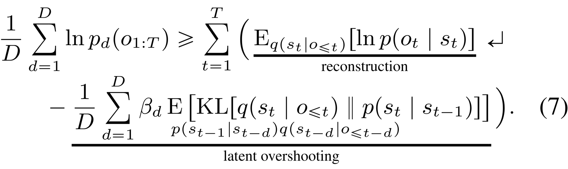
Latent overshooting can be interpreted as a regularizer in latent space that encourages consistency between one-step and multi-step predictions, which we know should be equivalent in expectation over the data set. We include weighting factors analogously to the -VAE
Experiments
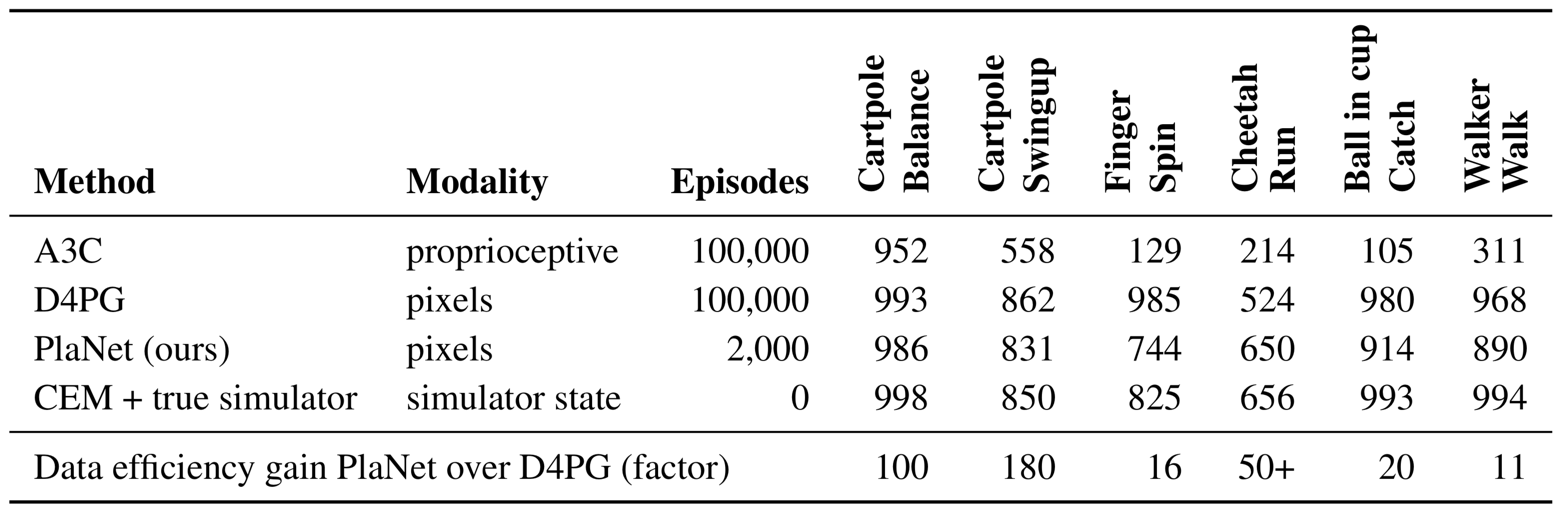
We evaluate PlaNet on six continuous control tasks from pixels. We explore multiple design axes of the agent: the stochastic and deterministic paths in the dynamics model, the latent overshooting objective, and online experience collection. We refer to the appendix for hyper parameters. Besides the action repeat, we use the same hyper parameters for all tasks. Within one fiftieth the episodes, PlaNet outperforms A3C
For our evaluation, we consider six image-based continuous control tasks of the DeepMind control suite

(b) The finger spin task requires predicting two separate objects, as well as the interactions between them.
(c) The cheetah running task includes contacts with the ground that are difficult to predict precisely, calling for a model that can predict multiple possible futures.
(d) The cup task only provides a sparse reward signal once a ball is caught. This demands accurate predictions far into the future to plan a precise sequence of actions.
(e) The simulated walker robot starts off by lying on the ground, so the agent must first learn to stand up and then walk.
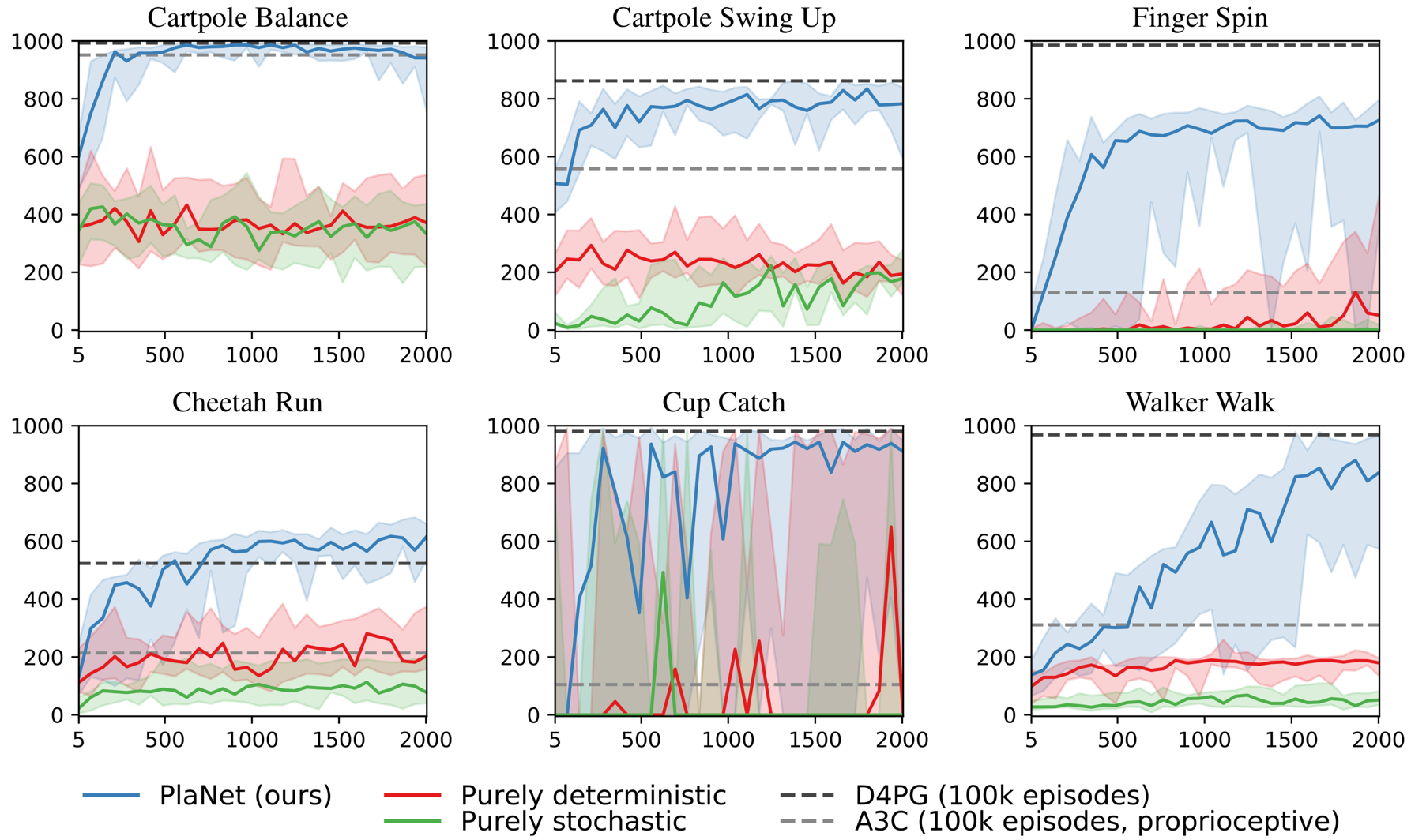
Comparison to model-free methods Figure 8 compares the performance of PlaNet to the model-free algorithms reported by
Model designs Figure 8 additionally compares design choices of the dynamics model. We train PlaNet using our recurrent state-space model (RSSM), as well as versions with purely deterministic GRU
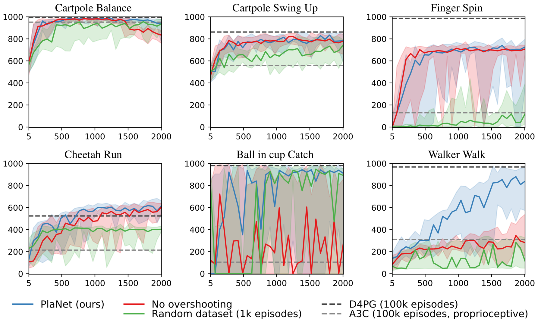
Agent designs Figure 9 compares PlaNet with latent overshooting to versions with standard variational objective, and with a fixed random data set rather than collecting experience online. We observe that online data collection helps all tasks and is necessary for the finger and walker tasks. Latent overshooting is necessary for successful planning on the walker and cup tasks; the sparse reward in the cup task demands accurate predictions for many time steps. It also slows down initial learning for the finger task, but increases final performance on the cartpole balance and cheetah tasks.
One agent all tasks Additionally, we train a single PlaNet agent to solve all six tasks. The agent is placed into different environments without knowing the task, so it needs to infer the task from its image observations. Without changes to the hyper parameters, the multi-task agent achieves the same mean performance as individual agents. While learning slower on the cartpole tasks, it learns substantially faster and reaches a higher final performance on the challenging walker task that requires exploration.
For this, we pad the action spaces with unused elements to make them compatible and adapt Algorithm 1 to collect one episode of each task every update steps. We use the same hyper parameters as for the main experiments above. The agent reaches the same average performance over tasks as individually trained agents. While learning is slowed down for the cup task and the easier cartpole tasks, it is substantially improved for the difficult task of walker. This indicates that positive transfer between these tasks might be possible using model-based reinforcement learning, regardless of the conceptually different visuals. Full results available in the appendix section of our paper.
Related Work
Previous work in model-based reinforcement learning has focused on planning in low-dimensional state spaces
Planning in state space When low-dimensional states of the environment are available to the agent, it is possible to learn the dynamics directly in state space. In the regime of control tasks with only a few state variables, such as the cart pole and mountain car tasks, PILCO
Hybrid agents The challenges of model-based RL have motivated the research community to develop hybrid agents that accelerate policy learning by training on imagined experience
Multi-step predictions Training sequence models on multi-step predictions has been explored for several years. Scheduled sampling
Latent sequence models Classic work has explored models for non-Markovian observation sequences, including recurrent neural networks (RNNs) with deterministic hidden state and probabilistic state-space models (SSMs). The ideas behind variational autoencoders
Video prediction Video prediction is an active area of research in deep learning.
Relatively few works have demonstrated successful planning from pixels using learned dynamics models. The robotics community focuses on video prediction models for planning
Discussion
In this work, we present PlaNet, a model-based agent that learns a latent dynamics model from image observations and chooses actions by fast planning in latent space. To enable accurate long-term predictions, we design a model with both stochastic and deterministic paths and train it using our proposed latent overshooting objective. We show that our agent is successful at several continuous control tasks from image observations, reaching performance that is comparable to the best model-free algorithms while using 50× fewer episodes and similar training time. The results show that learning latent dynamics models for planning in image domains is a promising approach.
Directions for future work include learning temporal abstraction instead of using a fixed action repeat, possibly through hierarchical models. To further improve final performance, one could learn a value function to approximate the sum of rewards beyond the planning horizon. Moreover, exploring gradient-based planners could increase computational efficiency of the agent. Our work provides a starting point for multi-task control by sharing the dynamics model.
If you would like to discuss any issues or give feedback regarding this work, please visit the GitHub repository of this article.